Understanding Central Tendency Measures | CFA Level I Quantitative Methods

Welcome back, future CFA champs! Let’s dive into the world of central tendency measures such as mean, mode, median, harmonic mean, and geometric mean. We’ll also explore quantiles and how to calculate them. Ready? Let’s go!

Population vs. Sample

First, let’s clarify the difference between a population and a sample. A population is the entire group of interest, while a sample is just a subset of it. Parameters describe population characteristics, while statistics describe sample characteristics.

Mean: Population Mean and Sample Mean

The population mean is the sum of all population values divided by the number of population members. The sample mean is calculated similarly for samples. The Greek symbol “mu” represents the population mean, while “x bar” represents the sample mean. Capital “N” denotes population size, and lowercase “n” denotes sample size.

Arithmetic Mean

Both population and sample means are arithmetic means, calculated by dividing the sum of observation values by the number of observations. If you imagine placing observations on a scale, the scale balances when the fulcrum is at the arithmetic mean. The sum of deviations from the mean is always zero.

Weighted Mean

Sometimes, you need to assign different weights to observations. To calculate the weighted mean, multiply each observation by its corresponding weight and sum them up.

Mode

The mode is the most frequently occurring observation. It’s useful for large sample sizes and helps identify the most prevalent observation. Distributions can be unimodal (one mode), bimodal (two modes), or trimodal (three modes).

The median is the middle value when observations are ordered. If there’s an even number of observations, the median is the average of the two middle values. The median is less affected by outliers than the mean.

Harmonic Mean

The harmonic mean is calculated by taking the reciprocal of each observation, summing them up, reciprocating again, and multiplying by the number of observations. It’s commonly used to calculate the average cost of shares purchased over time.

Harmonic Mean (H) = n / (1/x₁ + 1/x₂ + … + 1/xₙ)

where n is the number of values in the dataset, and x₁, x₂, …, xₙ are the individual values.

Geometric Mean

The geometric mean is calculated by multiplying all observations and taking the nth root, where n is the number of observations. It’s often used to calculate mean return or growth over multiple periods. When using geometric mean for returns, add 1 to each return value.

Geometric mean = = (X₁x X₂x … x X_n)^1/n

Quantiles

Quantiles are values that divide a dataset into equal intervals. There are several types of quantiles:

• Quartiles: Divide the dataset into four equal parts (25%, 50%, 75%); the 50% quartile is the median.
• Quintiles: Divide the dataset into five equal parts (20%, 40%, 60%, 80%).
• Deciles: Divide the dataset into ten equal parts (10%, 20%, 30%, …, 90%).
• Percentiles: Divide the dataset into hundred equal parts (1%, 2%, 3%, …, 99%).

Quantiles can be calculated using different methods, such as linear interpolation, depending on the software or the approach being used.

Box and Whisker Plot

To visualize a dataset based on quantiles, we can create a box and whisker plot. This type of plot is useful for identifying the distribution of the data, the presence of outliers, and the overall spread of the dataset.

In a box and whisker plot, a straight line extending from the left to the right, known as the whiskers, plots the range from the lowest observation to the highest observation in the dataset. The box represents the range from the lowest observation in the second quartile (25th percentile) to the highest observation in the third quartile (75th percentile), also known as the interquartile range (IQR).

A straight line through the middle of the box plots the median observation of the dataset. An “X” will mark the arithmetic mean of the dataset.

From this plot, we can observe that the lowest observation is farther away from the center than the largest observation. This suggests that the data might include more outliers on the low side, which may skew some measures of central tendency like the mean.

In some cases, an analyst may decide that outliers should be excluded from a measure of central tendency. One technique for doing so is to use a trimmed mean. A trimmed mean discards a stated percentage of the most extreme observations. For example, a 10% trimmed mean would discard the lowest 5% and the highest 5% of the observations, so only the middle 90% of the ordered observations are considered in the calculation of the trimmed mean.

Another technique is to use a winsorized mean. Instead of discarding the highest and lowest observations, we substitute a value for them. For example, to calculate a 90% winsorized mean, we would determine the 5th and 95th percentile of the observations. Any values lower than the 5th percentile will be substituted with the 5th percentile value, and any values greater than the 95th percentile will be substituted with the 95th percentile value. So in essence, all the observations are considered in the calculation of the mean, just that the extreme outliers are substituted with values that are not too extreme.

Box and whisker plots provide a useful way to visualize the distribution of a dataset, as well as to identify potential outliers and their impact on measures of central tendency. By using trimmed or winsorized means, analysts can better account for the presence of extreme values in their data analysis.

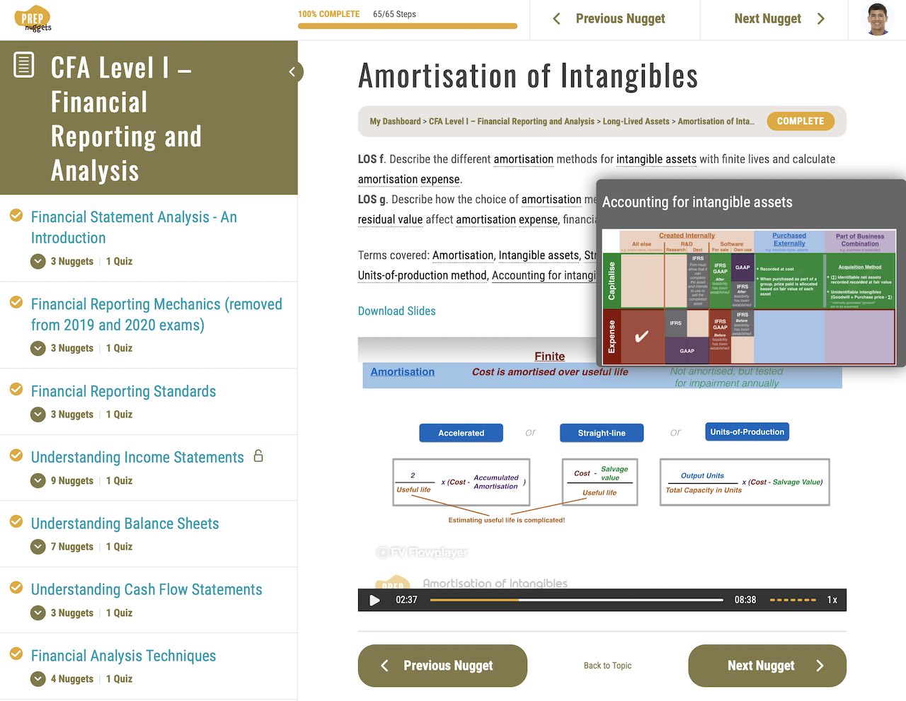
Conclusion

Measures of central tendency help describe the center point of a dataset, and different measures are appropriate for different situations. Understanding these measures is crucial for analyzing and interpreting data in various fields, including finance, economics, and statistics. Remember to practice using these measures and identifying when to apply each one!